Learning Visual Feedback Control for Dynamic Cloth Folding — What The Paper Does Not Tell You — Part 1 — Sensors
This is the first part of a technical report to provide more background on the design choices made in our paper “Learning Visual Feedback Control for Dynamic Cloth Folding”. Illustration by the excellent @davidbmulero
I was very pleased when I heard that the work I had poured my heart and soul into during my Master’s had been accepted for publication at the 2022 IEEE/RSJ International Conference on Intelligent Robots and Systems (IROS 2022).
What made me even more excited was when I found out we were among the few finalists for the Best Paper Award (out of 1716 accepted papers). Even though we didn’t win, it was great to see that the winner was a paper in the same field as ours: robotic cloth manipulation.
The purpose of this series of blog posts is to highlight some of the technical challenges we were able to overcome, but were not able to cover in detail in the limited number of pages the conference paper format allows. I also hope it is a fresh approach to describing what happens under the hood of creating a research paper, which often lack details on the engineering “a-ha” -moments most of us are actually driven by.
The Cloth Folding Problem
Robotic cloth manipulation is an important field since it has many potential applications in various industries. For example, robots that can manipulate cloth could be used in the clothing and textile industry to automate the manufacturing process, leading to increased efficiency and productivity.
It could also be used in the service industry, such as in hotels or hospitals, to automate tasks such as making beds or changing linens. Additionally, robots that can manipulate cloth can be used in research and development to test and improve materials and textiles for use in various applications.
In short, the ability to manipulate cloth has the potential to revolutionize a variety of industries and improve the efficiency and productivity of many tasks.
The Sim2Real Challenge
As highlighted, robots that can manipulate cloth can be very useful, but it’s a difficult task because there is a lot of variability in materials and they can move in many different ways. It’s especially hard to make a robot fold cloth neatly and quickly.
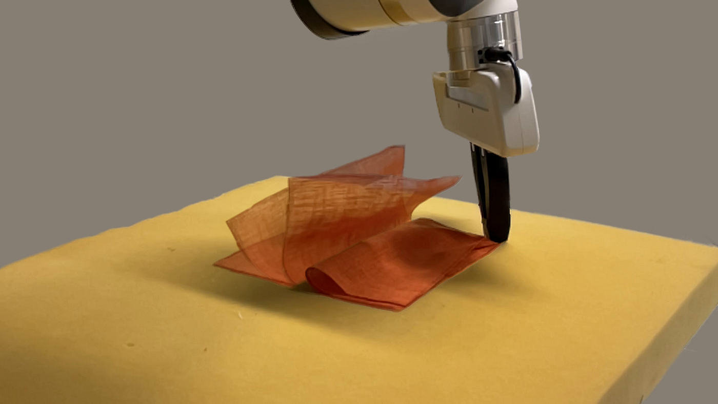
Dynamic cloth folding in action. Teaching robots skills in simulation and transferring them to the real world is hard. Photo by the brilliant @gokhanalcan_.
One way to help robots learn how to do this is to use a method called Reinforcement Learning (RL). RL can be used to let robots practice manipulation skills in a computer simulation, and then they can use what they learned to fold fabrics in the real world.
However, one of the main challenges in using a simulation to train robots for cloth folding is the so-called “Sim2Real gap.” This refers to the difficulty of transferring skills learned in simulation to the real world, where the robot must deal with all the complexities and uncertainties of the physical environment.
In the case of cloth manipulation, the Sim2Real gap can be especially pronounced due to the high dimensionality of the configuration space and the complex dynamics affected by various material properties. This means that it can be difficult to predict exactly how a piece of cloth will behave in the real world, and the robot must be able to adapt and adjust its actions accordingly.
To address the Sim2Real gap, it is important to use methods that can learn robust and generalizable policies that can perform well in a variety of different conditions. This can involve using techniques such as incorporating visual feedback and domain randomization to help the robot adapt to the real-world environment.
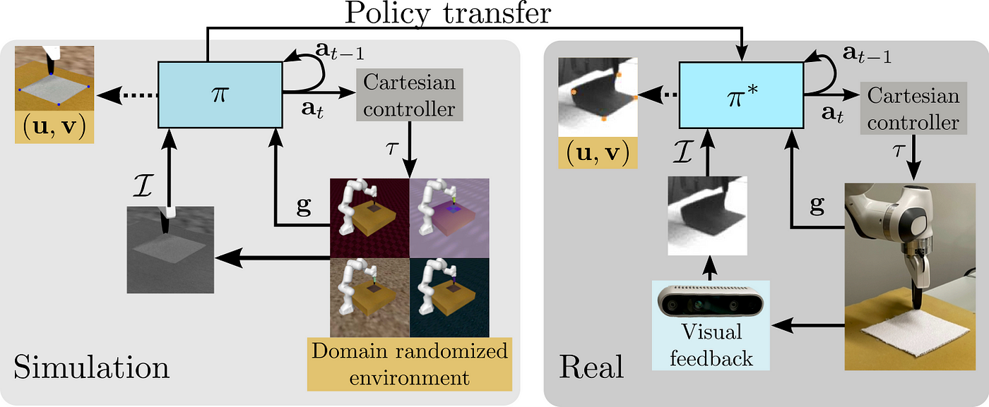
In our paper, we trained an RL model that dynamically folds various pieces of fabric using a robot and visual feedback. The theme of the technical challenges related to our work was aligning the robot and fabric behavior in simulation with their behavior in the real world. The main challenges were:
- Taking into account the constraints related to collecting visual feedback data in the real world, such as the type and frequency of data available from a camera
- Identifying a suitable and identical way to control the robot in both simulation and the real world
- Aligning the simulated and real environments manually in terms of visual attributes and dynamic behavior of the cloth is not feasible in practice
The first part of the blog series will describe how we were able to identify a suitable sensor and settings that allowed us to solve the dynamic cloth folding problem successfully. Parts 2 and 3 will describe identifying a controller, and aligning cloth behavior in simulation and the real world.
Sensor Frequency and Latency
Given the nature of the dynamic folding task, it was crucial to be able to control the robot as frequently as possible, since if deformations of the fabric are not accounted for fast enough during the manipulation, the task will be impossible to achieve since gravity will pull down the non-grasped part of the cloth.
The above is in contrast to a static manipulation task, where the robot could in theory move arbitrarily slow with a low frequency, and the task would still be successful since the velocity and acceleration of the robot do not affect the end result.
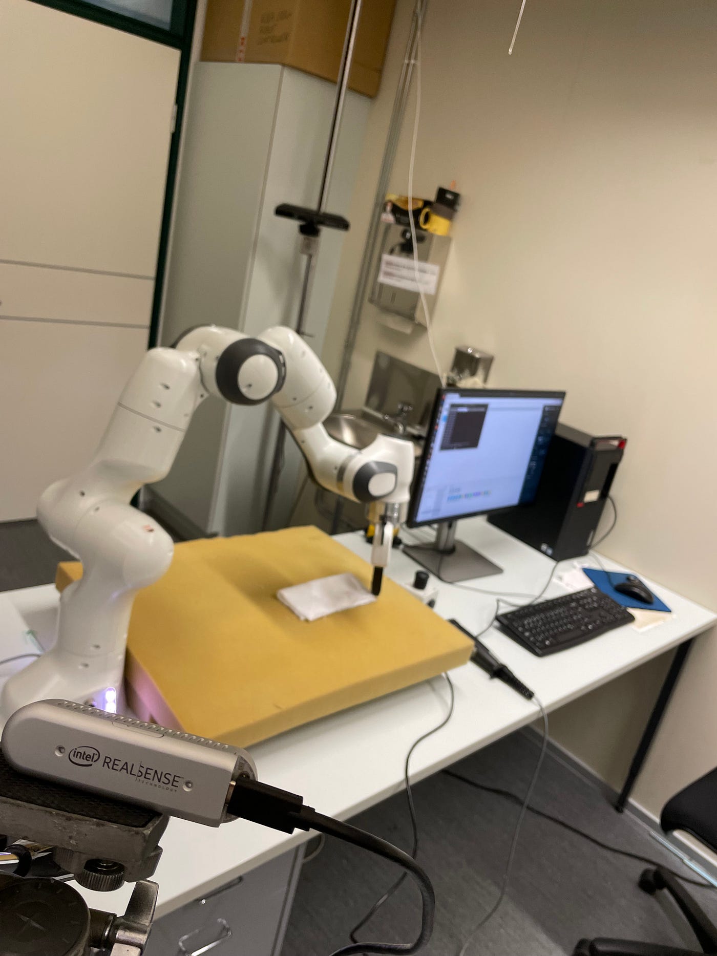
The lab setup. We used an Intel RealSense D435 to capture feedback. Photo by the author.
A limiting factor in how high of a frequency can be used for providing feedback in closed-loop control is the frequency of the sensor providing feedback. Especially if the feedback is visual, it is unlikely that the robot controller can be provided with new feedback at every update, since most cameras operate at a much lower frequency than the robot’s controller. Therefore interpolating the control signal between receiving new feedback becomes an important design choice.
Another aspect related to cameras besides their operating frequency is the latency they experience. Latency can be understood as the time between capturing the observation and actually having it available to be used in a downstream task such as an RL policy. It is therefore not enough for a camera to operate fast enough in terms of frequency, but also the content of the feedback should be recent enough. A camera may be able to output images at as high as 300 frames per second, but if the frames are delayed by e.g. a second, it would force using a frequency lower than 1Hz to keep things markovian.
Evaluating the RealSense D435
Our lab had a few sensor options available, including the Intel RealSense D435, which is a popular option in the RL community due to its commercial availability and a reasonable price. Intel also provides a robust SDK for interfacing with its RealSense devices. There is also a Python wrapper for the SDK, which was a nice feature for quick debugging and learning, but the main interest was towards the C++ API since the real-world robot control system would use it instead of Python.
The first thing in evaluating the usefulness of the RealSense D435 was to evaluate the different output streams available along with their frequencies and latencies since they have big implications on the RL algorithm and control side. The main output streams considered were a pure RGB-based stream, along with an infrared-based stream, which provides grayscale images of the environment. The camera also has a stereo depth sensor but using it was outside of the scope of the paper.
The frequency of the camera is measured as frames per second (fps) and can accurately be set using the SDK. However, estimating the latency of a camera is not a straightforward task. Fortunately for the RealSense camera, there is an open-source tool called rs-latency-tool, which allows estimating the latency empirically.
Measuring latency
The rs-latency-tool encodes the current wall clock time into binary form and displays the bits as white dots on the screen as shown below. The camera is then pointed at the screen, and the tool starts capturing frames of the screen, where the frames include the metadata of when they were captured in wall clock time.
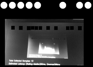
The rs-latency-tool. Photo by author.
A computer vision algorithm is then applied to the captured frames in a separate thread, which decodes the wall clock time back from binary form. After extracting the wall clock time of the frames, it can be compared to the wall clock time in the metadata. The difference between the two times is then considered as an estimate of the latency.
The latency tool worked very well in most cases for both the RGB and infrared streams, but we noticed that with some image resolutions the algorithm was unable to detect the points, which made a thorough evaluation of all available image resolutions a challenge.
A modified version of the latency tool. Photo by the author.
Given the issues with detection robustness, we decided to modify the latency tool slightly, where the tool would render the current wall clock time in a human-readable form instead. The camera was then pointed again towards the screen so that the camera was capturing the rendered wall clock time next to the displayed wall clock time. Snapshots displaying the captured call clock time and current wall clock time were captured and saved by using the screen capture functionality provided by the operating system. Visual inspection of the captured images then allowed us to get a rough estimate of the latency.
Finding an acceptable level of latency
In order to get an estimate of the maximum allowable latency for the camera, the RL training of the agent was run using our simulation environment (more details provided in parts 2 and 3), where the number of simulation environment steps between providing new feedback and a new position for the gripper was varied. In the training runs, the gripper could move arbitrarily in 3D space, which made it slightly unrealistic compared to the real world with an actual controller but still provided a rough estimate of how often feedback needs to be provided.
Training runs were run with new feedback frequencies of 5Hz, 10Hz, and 20Hz, with 100x100 pixel grayscale images. The image size is a common choice for training convolutional neural networks (CNN), where image sizes larger than 100x100 pixels can make training very slow with off-the-shelf hardware. After running all variants with different random seeds for a few runs, the results showed that a feedback frequency of 10Hz was the lowest that could be used to learn the folding task consistently.
The above meant that the allowable latency of the camera could be 100ms at maximum, where the captured feedback would still include signal related to the previously executed action.
Arriving at a feedback modality
Based on initial tests, the RGB stream of the RealSense D435 proved unsuitable for our purposes, since the estimated latencies were on average around 120ms. Therefore using the infrared sensor was the only option left to discover. Fortunately, Intel had published a paper along a new version of firmware for the D435 device, which allowed a high-speed capture mode of 300 fps of the infrared streams compared to the previous maximum of 60 fps.
The frequency of the camera was not really an important factor, since, in theory, 10 fps would suffice for the required 10Hz feedback frequency. However, it turns out that the frequency and the latency of the camera are related: a higher frequency also results in lower latency.
According to the paper, the 300 fps mode could achieve a latency between 25 and 39 milliseconds, which is sufficient given the 100ms maximum. The 300fps mode also provided 848x100 pixel frames, which also accommodated the 100x100px requirement of the RL policy.
Additional sources of latency
In addition to the latency of the camera itself, latency caused by communicating frames to the RL policy, and the policy communicating actions to the robot controller had to be taken into account as well.
The robot we used (Franka Emika Panda, more details in part 2) used an internal control loop of 1kHz, which means that even with the 300 fps feedback capture, the camera would be blocking the execution of the controller’s 1kHz loop if waiting for new frames was placed in the control loop.
The real robot’s controller was built using the Robot Operating System (ROS), which provides a standardized, ethernet-based messaging channel between different nodes. Given the mismatch between the controller and sensor latencies, it was therefore a natural choice to create a separate ROS node for the camera and the RL policy inference, and let it communicate with the controller node via ROS.
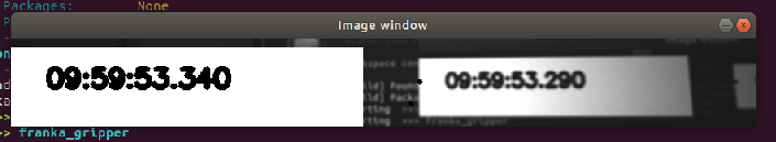
In order to measure the combined latency of the camera, the RL policy, and any extra delay caused by ROS, the custom latency tool was further modified to be a ROS node itself, which received images as ROS messages and displayed the received image along with the current wall clock time identically to the initial modified latency tool.
The created camera node then ran the image-capturing and RL policy inference loop in its own process and sent it to the latency tool node via ROS. The snapshots captured of the output from the latency tool node thus included both the latency inherent in the camera and extra latency that was caused by the rest of the system.
With the above setup, the observed mean latency was roughly 50ms, with a range from 35ms to 60ms. This empirical result verified that the 848x100px at 300fps -setting could be used to provide feedback to the controller at a lower than 100ms latency.
Conclusion
This blog post covered the details on how we were able to find a suitable sensor and feedback modality for our paper “Learning Visual Feedback Control for Dynamic Cloth Folding”. Parts 2 and 3 will further describe design choices related to the controller and simulation environment.
The links to all of the blog posts in the series can be found here: Part 1, Part 2, and Part 3.