Tutorial: How to Build a Simple Neural Network in Rust

The example code can be found here

Image generated by DALL-E

Introduction

Neural networks have experienced a surge in popularity, captivating data scientists and machine learning practitioners worldwide. However, while these experts excel at data modeling and analysis, their proficiency in writing reliable and scalable software systems may be limited. As neural networks become increasingly prevalent in real-world applications, it becomes crucial for software engineers to bridge the gap between mathematical understanding and robust code implementation.

In this rapidly evolving era of machine learning, the demand for neural networks in real-world applications has skyrocketed. Traditionally, Python has been the language of choice due to its simplicity and extensive ecosystem. However, as the complexity of these applications grows, so does the need for more reliable and performant code.

The Limitations of Python and the Appeal of Rust for Machine Learning

Python, having a huge ecosystem of data science and machine learning libraries and a shallow learning curve, is the go-to choice for most data scientists and machine learning engineers. However, its lack of static typing can lead to subtle bugs and hinder long-term code maintenance. Additionally, Python often relies on bindings to lower-level languages like C++ for computationally intensive tasks, introducing complexities and potential issues during integration.

Enter Rust — an opportunity to write high-level, readable code with the benefits of static typing and memory safety. Its zero-cost abstractions and advanced compiler optimizations ensure efficient execution, making it well-suited for both small-scale experiments and large-scale production systems. Rust’s ability to create native libraries allows heavy computations to be performed directly within the language, eliminating the need for external bindings and simplifying the development process.

Tutorial: Building a Simple Fully Connected Neural Network in Rust

In the following sections, we will dive into a tutorial on how to write a simple fully connected neural network in Rust. This tutorial serves as a practical example for software engineers to gain a clear understanding of the mathematical principles behind neural networks and how they can be implemented in code.

Throughout the tutorial, we will cover key concepts such as forward and backward propagation, (stochastic) gradient descent, and the loss function. By following this step-by-step guide, you will not only enhance your knowledge of neural networks but also realize that data science tasks can be accomplished in languages other than Python, serving as a valuable refresher for machine learning engineers.

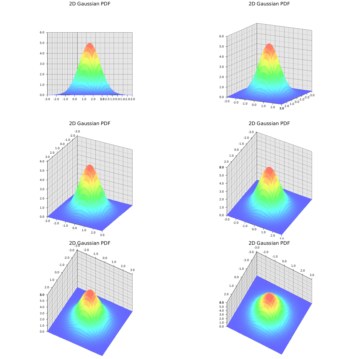
The standard 2D Gaussian we are trying to learn. Gif by the author.

Learning in Neural Networks

In this section, we will explore the process of learning in neural networks step by step. We’ll analyze the example code and explain the underlying math involved at each stage. We can start by looking at the main.rs script to get a high-level view of the training loop.

Inputs and Targets

First, for each training iteration we generate random input samples x within the range [-3.0, 3.0]. These samples are represented as a 2-dimensional array, where each row corresponds to a single input instance. Additionally, we compute the target values for the input samples using the standard 2D Gaussian PDF function, which calculates the probability density function based on the input coordinates.

Forward Pass

Next, we perform a forward pass through the neural network by calling the forward method of the neural network (nn). This operation propagates the input data x through the network's layers, producing the predicted output y. Each layer applies linear transformations (weight multiplication) followed by non-linear activation functions to generate the output activations.

Loss Calculation

Once we have the predicted output y, we compute the loss value by invoking the forward method of the mean squared error (MSE) loss function (loss). The loss function compares the predicted output y with the target values and calculates the squared differences between them. The resulting loss value represents the discrepancy between the predicted and target values.

Backward Pass

To update the network’s parameters and improve its performance, we need to compute the gradients of the loss with respect to the network’s parameters. We start by calling the backward method of the loss function to obtain the derivative of the loss with respect to the predicted output (dL_dy). This derivative represents the sensitivity of the loss to changes in the predicted output.

Next, we invoke the backward method of the neural network to compute the gradients of the loss with respect to the network's parameters. This operation involves the chain rule, where the gradients are calculated by propagating the derivative dL_dy backward through the layers of the network. The gradients capture how changes in the network's parameters affect the loss. If you are not familair with backpropagation from before, the great Andrej Karpathy has created a wonderful introduction video on the topic.

Parameter Updates

After computing the gradients, we update the network’s parameters using stochastic gradient descent. The learning rate (learning_rate) determines the step size in the parameter update process. We adjust the learning rate over time to gradually decrease the step size for more fine-grained optimization.

The network’s parameters, including weights (W) and biases (b), are updated by subtracting the product of the gradients and the learning rate from their current values. This process iteratively refines the network's parameters to minimize the loss and improve the accuracy of the predictions.

Throughout the training loop, we monitor the progress by calculating the average loss over a specified number of iterations. This provides insights into how the network is learning and converging towards the desired solution.

By following this iterative process of forward pass, loss calculation, backward pass, and parameter updates, neural networks can gradually learn from data and improve their performance on a given task.

Unveiling the Components: Exploring the Inner Workings

While the abstractions provided by neural network libraries are undoubtedly convenient, it’s often beneficial to understand what goes on under the hood. In this section, we will take a closer look at the specific components involved in the learning process. By delving into the details of the neural network structure, the loss function, nonlinearity, and the linear layer, we can gain a deeper understanding of how these elements contribute to the overall functioning of the network.

Neural Network Structure

Photo by Hulki Okan Tabak on Unsplash

The neural network structure is a fundamental component that defines the architecture and connectivity patterns of the network. In this section, we will explore the neural network structure used in the code snippet provided. You can refer to the complete example here.

The NN struct represents the neural network and contains the layers and activation functions.

In the example, the neural network consists of three linear layers and two rectified linear unit (ReLU) activation functions. The layers are defined given a vector of hidden sizes.

The LinearLayer struct represents a linear layer, which performs a linear transformation on the input data. The ReLU struct represents the ReLU activation function.

The forward method performs a forward pass through the neural network, applying the linear transformations and activation functions to the input data:

The backward method performs a backward pass through the neural network, propagating the gradients and updating the parameters during training:

The Loss Function

Photo by István Jánka on Unsplash

The loss function is a crucial component in training a neural network. It quantifies the discrepancy between the predicted output and the desired target output, providing a measure of how well the network is performing. In this section, we will explore the Mean Squared Error (MSE) loss function implemented in the provided code.

The MSE struct represents the MSE loss function:

The dL_dx field stores the gradient of the loss function with respect to the input x. It is an Option type to accommodate scenarios where the backward pass is called before the forward pass.

The MSE struct follows the same forward/backward API as the rest of the components and has the following methods:

The get_output static method calculates the output of the MSE loss function for a given predicted output x and target output target:

Here, the error between the target output and the predicted output is computed by subtracting x from target. The mean squared error (MSE) is then calculated by squaring each element of the error, taking the mean, and returning the result.

The forward method performs a forward pass through the MSE loss function. It takes the predicted output x and the target output target as inputs:

In the forward pass, the gradient dL_dx is calculated as 2 * (x - target) / N, where N is the number of elements in x. This gradient represents the derivative of the loss with respect to the predicted output. It is then stored in the dL_dx field for later use in the backward pass. Finally, the output of the MSE loss function is obtained by calling the get_output static method.

The backward method performs a backward pass through the MSE loss function:

Here, the dL_dx gradient stored in the self.dL_dx field is returned. It represents the gradient of the loss function with respect to the input x. If the forward method is not called before the backward method, an error will be raised.

Nonlinearity — Rectified Linear Unit (ReLU)

Photo by Jr Korpa on Unsplash

The activation functions play a crucial role in introducing nonlinearity to the neural network, allowing it to learn complex relationships between inputs and outputs. In this section, we will explore the Rectified Linear Unit (ReLU) activation function implemented in the provided code.

The ReLU struct represents the ReLU activation function:

The dy_dx field stores the gradient of the activation function with respect to the input x. It is an Option type to accommodate scenarios where the backward pass is called before the forward pass.

It sets the dy_dx field to None, indicating that the gradient is not yet computed.

The get_output method calculates the output of the ReLU activation function for a given input x:

Here, the ReLU function is applied element-wise to the input x. The ReLU function returns the input value if it is positive, and 0 otherwise. This effectively removes negative values from the input, introducing nonlinearity to the network.

The forward method performs a forward pass through the ReLU activation function. It takes the input x as an argument:

In the forward pass, the gradient dy_dx is calculated by mapping over the elements of x. If an element is greater than 0, the derivative is set to 1; otherwise, it is set to 0. This gradient represents the derivative of the ReLU activation function with respect to the input x. It is then stored in the dy_dx field for later use in the backward pass. Finally, the output of the ReLU activation function is obtained by calling the get_outputmethod.

The backward method performs a backward pass through the ReLU activation function:

Here, the gradient of the loss with respect to the output dL_dy is multiplied element-wise with the dy_dx gradient stored in the self.dy_dx field. This calculates the gradient of the loss with respect to the input x, which is the result of the backward pass.

The Linear Layer

Photo by Martin Sanchez on Unsplash

The linear layer is a fundamental building block of a neural network, performing a linear transformation on the input data. In this section, we will examine the LinearLayer struct implemented in the provided code.

The LinearLayer struct represents a linear layer in a neural network:

The fields of the LinearLayer struct include:

W: The weight matrix of shape (out_features, in_features) representing the connections between the input features and the output features.
b: The bias matrix of shape (out_features, 1) representing the bias terms added to the linear transformation.
dL_dW: The gradient of the loss with respect to the weights W. It is an Option type to accommodate scenarios where the backward pass is called before the forward pass.
dL_db: The gradient of the loss with respect to the biases b. It is an Option type to accommodate scenarios where the backward pass is called before the forward pass.
dy_dW: The gradient of the output with respect to the weights W. It is an Option type to store the input values x for later use in the backward pass.

Here, the weight matrix W is initialized with random values of shape (out_features, in_features), and the bias matrix b is initialized with random values of shape (out_features, 1). The gradients dL_dW, dL_db, and dy_dW are set to None initially.

The get_output method calculates the output of the linear layer given the input x, weights W, and biases b:

Here, the input x is transformed using the weights W and biases b using matrix multiplication and addition. The result is then transposed to match the shape of the input x and returned.

The forward method performs a forward pass through the linear layer. It takes the input x as an argument:

In this method, the input x is stored in the dy_dW field for later use in the backward pass. Then, the get_output static method is called to calculate and return the output of the linear layer.

The backward method performs a backward pass through the linear layer. It takes the gradient of the loss with respect to the output (dL_dy) as an argument:

In this method, the gradient of the loss with respect to the weights W is calculated using matrix multiplication and transposition. The gradient of the loss with respect to the biases b is calculated by multiplying the transpose of dL_dy with a matrix of ones of the appropriate shape. The gradients dL_dW and dL_db are stored for later use. Additionally, the gradient of the loss with respect to the input (dL_dx) is calculated by multiplying dL_dy with the weights W and returned.

With these components, you can create and utilize a linear layer in a neural network for forward and backward passes.

Running the Full Example

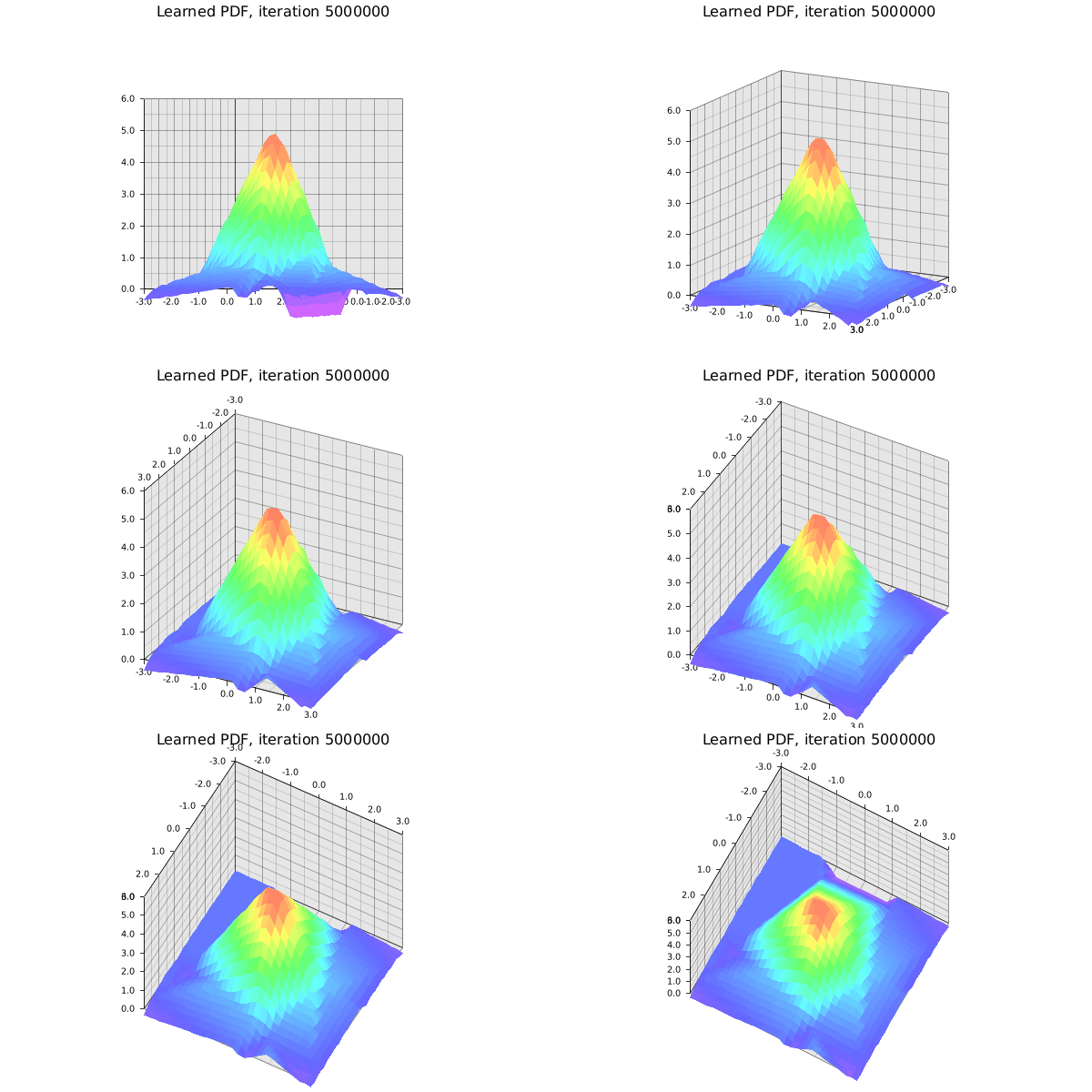
The learned standard 2D Gaussian. It’s not perfect given the small toy network and manually tuned hyperparameters. Gif by the author.

To recap, in this tutorial we constructed a simple neural network consisting of linear layers, rectified linear unit (ReLU) activation functions, and a mean squared error (MSE) loss function. The goal is to train the network to approximate a standard 2D Gaussian probability density function (PDF).

During training, we perform the following steps in each epoch:

Generate random input values (x) and target values based on the provided PDF.
Pass the input through the linear layer to obtain the output.
Apply the ReLU activation function to the output.
Calculate the loss by comparing the activation output to the target values using the MSE loss function.
Backpropagate the gradients through the network by sequentially calling the backward methods of the loss function, activation function, and linear layer.
Update the weights and biases of the linear layer using gradient descent: W -= learning_rate * dL_dW and b -= learning_rate * dL_db.

We repeat these steps for the specified number of epochs and print the loss every 100 epochs to monitor the training progress.

By optimizing the weights and biases through backpropagation and gradient descent, the neural network gradually learns to approximate the PDF. The training process aims to minimize the difference between the network’s output and the target values.

By running the example, you should see the following logs of the loss:

Iter 0, loss: 0.5877961461896624
Iter 10000, loss: 0.19003256083155048
Iter 20000, loss: 0.17370678307228338
Iter 30000, loss: 0.17006484610302272
Iter 40000, loss: 0.1636592581597393
Iter 50000, loss: 0.16056050672345717
Iter 60000, loss: 0.15110016510494112
Iter 70000, loss: 0.07819787045646279
Iter 80000, loss: 0.030993960636040124
Iter 90000, loss: 0.01961861500075111
Iter 100000, loss: 0.01631658998415742
Iter 110000, loss: 0.01509240837788267
...

We can see that the loss converges to around ~0.015 after ~100k iterations. Further tuning of the hyperparameters and increasing the network size will be required to achieve better performance. It is worth to note that neural networks are sensitive to exploding and vanishing gradients, which should be taken into account when making the network more complex.

Overall, this example demonstrates the basic workflow of training a neural network, including forward propagation, backpropagation, gradient descent, and updating the model’s parameters. You can further enhance this example by introducing more complex network architectures, different activation functions, or exploring advanced training techniques such as regularization or adaptive learning rates.

You can find the full example code in my crabnet repository on Github.